Complex Magic, Part 3: Function Evaluation via Integration

Accurate evaluation of the function is a classic problem in numerical analysis. This function can be seen as an approximation to the first derivative of at , . More generally, is the divided difference of at and and this fact combined with our discussion of catastrophic cancellation due to roundoff in divided differences in a previous post (Complex Magic, Part 1) should trigger an alarm.

The “usual” accurate method to evaluate is to instead evaluate , unless , in which case the result is set to 1, given that, say for continuity, is defined to be 1. This is the method employed in MATLAB’s expm1 whose implementation is based on an algorithm due to William Kahan.

Why do and , which are equal in exact arithmetic for all , evaluate differently in floating point arithmetic? The reason may be rigorously explained with a floating point error analysis; see Nick Higham’s ASNA, for example. The difference of and , in floating point arithmetic, is that the former, by design, enjoys a cancellation of errors in division that the latter does not. Note that neither the numerator nor the denominator of can be evaluated accurately in floating point arithmetic. For x = 9.000000000000000e-015, using double precision in MATLAB R2009a on a machine running Windows XP with an Intel Core 2 Duo E8400 CPU, the former is 9.103828801926284e-015 and the latter is 9.103828801926243e-015, while in exact arithmetic they are, up to 16 significant digits, 9.000000000000040e-015 and 8.999999999999999e-15, respectively. The ratios, however, are both equal to 1.000000000000004 up to 16 significant digits!

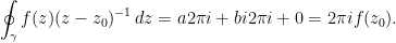
From the title of this post, and the fact that the method just illustrated was referred to as “usual,” it shouldn’t be too hard to expect that another method is to be discussed here. The underlying idea of this other method, due to [KassamTrefethen2005], is the same as the one discussed in Complex Magic, Part 2: Cauchy’s integral formula, only this time Cauchy helps with calculating the function itself, not its derivative,

An elegant heuristic proof of (1), based on a fluid flow interpretation from Mark Levi’s Mathematical Mechanic [Levi2009], can be given by recasting the definition of holomorphicity of the function at , namely that there exists such that

(in other words, namely that there exists a linear approximation to at ) as the linear combination of a source generating function, , a vortex generating function, , and an ideal (incompressible and irrotational) flow generating function, ,

noting that the contributions of these three terms to the contour integral are , , and , respectively, and finally summing up these contributions to get

– The word “generating” is important in the above “proof.” The source, vortex, and ideal flow functions arise from treating the complex conjugates of the aforementioned generating functions as vector fields.
– Donald Knuth’s “” Calculus letter to Notices of the American Mathematical Society [PDF, TeX] offers a lively discussion on , and , notation.

With only a slight modification (the highlighted lines) to the diffc of Complex Magic, Part 2 we can get it to work for zeroth derivative (i.e., function evaluation), too.

function [S_M,delta_M] = diffc(f,varargin)

[x0,n,r,M] = deal(0,1,.1,3);

optArgs    = {x0,n,r,M};
emptyArgs  = cellfun(@isempty,varargin);
[optArgs{~emptyArgs}] = varargin{~emptyArgs};
[x0,n,r,M] = optArgs{:};

f_x0      = f(x0);
[G_M,S_M] = deal(0);
for m = 1:M

    if n == 0
        mn = M;
        mobius_m = 1;
    else
        mn = m*n;
        mobius_m = mobius(m);
    end

    t   = linspace(1/(mn),1,mn);
    g   = real( f( x0 + r * exp(1i * 2*pi * t) ) );

    G_M = max( abs( [G_M f_x0 g] ) );
    S_M = S_M + mobius_m * ( mean(g) - f_x0 );

    if n == 0, break, end
end

delta_M = eps(G_M) * G_M/S_M;
S_M     = factorial(n)/(r^n) * S_M;

Apropos of nothing, note that because linspace(d1,d2,n)‘s implementation outputs [d1+(0:n-2)*(d2-d1)/(floor(n)-1) d2], there is always at least one point, namely d2, returned by linspace, even if n = 0. Also, note that apparently the method MATLAB uses for printing the values of symbolic variables in the Command Window is different from what it uses for double variables, as there is no indentation when symbolic variables are output to the Command Window. Compare x = 1, y = sym(1), z = vpa(1).

f = @(x) (exp(x) - 1)./x;

x_0 = 1e-18; x_vpa = vpa(x_0,32); n = 0; r = .5; M = 16;
tic, f_vpa         = f(x_vpa),              toc
tic, [f_M,delta_M] = diffc(f,x_0,n,r,M),    toc

We see from the output of the above snippet that, using variable precision arithmetic (vpa) with 32 digits, the value of for x = 1e-18 is 1.0000000000000000004999535947385 and that on a contour of radius using only points for the trapezoidal quadrature, diffc achieves 1.000000000000000 which agrees with the vpa evaluation in all its 16 digits.

The integrand in (1) was written as , and not the conventional . Why would we want to do that?

-----BEGIN DIGRESSION-----

Let us digress, a bit and not to the Neverland! According to Gilbert Strang, there are only two functions whose power series one should know by heart: and . Let’s not touch the former, lest we digress too much and get lost! As for the latter, recasting it as allows its power series to be written with the familiar form

for ‘s that can come from different fields ; in particular can be a scalar or a square matrix and (2) stays intact. As an aside, it is noted that (2) may be used, formally, to discover the formula for for the more general case of one-sided inverses in rings. More on this may be read in How to Construct .

Another place this kind of recasting can yield a unified treatment is in projections. For and elements of a vector space over the complex field , the projection of over is usually written as , with denoting the Hermitian (complex conjugate) transpose of . Recasting this as makes this expression identical to the one that holds in the more general case when is a matrix and the projection is into a subspace of spanned by the columns of (that is, the column space of ).

-----END DIGRESSION-----

A similar rationale is behind recasting the integrand in (1) from the usual division to multiplication by the inverse: the latter holds in the more general case when is a square matrix, with the slight modification of to , where is the multiplicative identity of the field . The contour has to enclose the eigenvalues of —if is a scalar (that is, if is the complex field ) its eigenvalue is itself, as .

Why is the operator so important? Because it appears in many important numerical methods. One of the places that it appears is in Exponential Time Differencing (ETD) schemes; see, for example, [CoxMatthews2002]. ETD schemes are particularly useful when solving stiff PDEs. Discretizing the spatial dimension of a PDE, the result may be written as a system of ODEs of the form

where and are the discretized linear and nonlinear parts of the original PDE, respectively. (For instance, supposing that denotes state variables of a mechanical system, and could be the normalized, linear and nonlinear forces acting on the system, respectively. If the constitutive laws are imposed, via a matrix and nonlinear function for the linear and nonlinear parts of (3), normalization can be dropped from the the previous statement.) When the eigenvalues of have very different magnitudes—either because there is a very negative eigenvalue, indicating strong damping (exponential decay) as in dissipative systems, or because there is a large imaginary eigenvalue, indicating rapid oscillations as in dispersive systems—the system (3) is categorized as stiff. (It is assumed that is “normal” so that analyzing its eigenvalues gives us a true prediction of what it represents. Let’s not enter the world of pseudospectra at this time.) It is noted that a differential equation has attached to it a differential operator whose definition is not complete without the necessary initial conditions. As a result, the notion of stiffness depends not only on the bare system of differential equations but also on the initial conditions. Furthermore, many problems are not initially stiff; they become stiff only when the solution approaches a certain state.

In a stiff system of ODEs two restrictions apply to the time steps a numerical solver can take; one is imposed by stability, dictated by the largest eigenvalue (in magnitude), just as in the case of a single ODE, and the other is imposed by the desired accuracy. The former pushes the time step to be much smaller than is required by the latter and this is a dilemma. A scheme not specially designed to handle stiffness is not aware of these two different time scales, would take very small steps and as a result would take an awfully long time to solve the a stiff problem. It is important to note that this (time) inefficiency is the only problem such a scheme would have; other things being equal, stiffness does not render a nonstiff scheme unstable or divergent. (See Cleve Moler’s “corner” article Stiff Differential Equations and Gilbert Strang’s treasure trove “Introduction to Applied Mathematics” for more details.)

The discussion of ETD here is based on [CoxMatthews2002], which is a very nice read. The underlying idea of ETD schemes is simple: apply the matrix exponential to (3) and approximate the resulting integral. ( is an integrating factor for the linear part of (3) so the integral to approximate is coming from the nonlinear part.) Over a single time step of length from to this gives

A first order approximation to already brings out the notorious in (4)

where and denotes an approximation to . With higher order approximations, we have higher order versions of and the resulting cancellations due to roundoff are more sever. For example, here is Cox and Matthews ETD4RK, a fourth-order ETD scheme with Runge-Kutta time stepping:

(The terms multiplying powers of in the above equations are prone to severe cancellation due to roundoff.)

We are now ready to write a simple function fevalc that computes (1) for the general case that is a matrix:

function f_z0 = fevalc(f,varargin)

[z0,r,M]  = deal(0,.1,16);
optArgs   = {z0,r,M};
emptyArgs = cellfun(@isempty,varargin);
[optArgs{~emptyArgs}] = varargin{~emptyArgs};
[z0,r,M] = optArgs{:};

I    =   eye(size(z0));
f_z0 = zeros(size(z0));

zs = r * exp( 1i*pi*( ((1:M) - .5 )/M ) );
for j = 1:M
    z = zs(j);
    zI_z0_inv = inv(z*I - z0);
    f_z0 = f_z0 + f(z) * zI_z0_inv * z; %#ok<MINV>
end
f_z0 = real(f_z0)/M;

Note that for the special case when is a scaler this function is equivalent to the one-liner zs = r * exp( 1i*pi*( ((1:M) - .5 )/M ) ); f_z0 = real(mean(f(zs))).

For the sake of demonstration, let us calculate one of the “troubled” terms (or “troublesome,” depending on your view point!), say , in (5) when the time step is and is the second-order, Chebyshev differentiation matrix for a problem with constant Dirichlet boundary conditions:

function ETD4RK_term_eval
N  = 5;
D  = cheb(N);
h  = 1/10;
D2 = D^2; D2 = .01*D2(2:N,2:N);
Ah = h*D2;
f  = @(z) ( h*z^(-3) * (-4 - z + exp(z)*(4 - 3*z + z^2) ) );

f_A   = f(Ah);
f_A_c = fevalc(f,Ah,20,10);

function [D,x] = cheb(N)

if N == 0, D = 0; x = 1; return, end
x = cos(pi*(0:N)/N)';
c = [2; ones(N-1,1); 2].*(-1).^(0:N)';
X = repmat(x,1,N+1);
dX = X - X';
D  = (c*(1./c)')./(dX + (eye(N+1)));
D  = D - diag(sum(D,2));

(The border rows and columns are being chopped off from D2 to impose the constant boundary conditions. For more details about the implementation of boundary conditions and how the function cheb generates the Chebyshev differentiation matrix see [Trefethen2000].)

This is calculated by direct substitution, which is completely off,

This is calculated using fevalc

Of course, as mentioned before, the calculation in ETD4RK_term_eval is for demonstration only. The “troubled” terms in (5) need not, and in fact should not, be calculated one by one using fevalc, as the inverse matrix is shared among them and need be calculated only once. Furthermore, because these terms have powers of , the multiplication by in ETD4RK_term_eval can be accounted for by reducing the power of by , instead of actually doing the multiplication. Refer to [KassamTrefethen2005] for more details. As an aside, it is noted that this is one of the very rare cases that the inverse matrix itself is needed; no system of linear equations is being solved and as a result what inv is doing cannot be achieved using the backslash operator. Another case in which the inverse matrix itself is needed and cannot be replaced by the backslash operator is calculating the standard errors of the estimates, in an identification problem, based on the inverse of the Fisher information matrix.